
 rrdtool is a powerful tool to store time series data and create graphs. It is very easy to create your first simple graph. This how-to will show the quickest way to generating your first graphs while explaining the options used.
rrdtool is used in many monitoring solutions. Its one of the easiest and best ways to store datapoints and generate graphs from them.
Creating an rrd database file
Before we start to generate the first graph, we need an rrd database file with data in it.
$ rrdtool create dbfile1.rrd --step=1 --start=now-1000s \
    DS:ds1:GAUGE:1:U:U \
    RRA:AVERAGE:0.5:1:1000
The above command will “create” an rrd database file named “dbfile1.rrd” with an expected step size of “1” second (–step=1). That means, this rrd database file expects one entry every second. With the “–start” parameter, the start time for the rrd database file is set to 1000 seconds in the past. Details for the syntax to define the start time can be found at rrdtool -> rrdgraph_examples -> Time ranges.
The line starting with “DS:” represents the “data set” to be stored in the database file. In short, the definition of the data set is a colon “:” separated list. After the “DS” keyword, the data set name (“ds1”) is specified (second element). The third element is the data set type which is chosen to be GAUGE for that example. A detailed description of data set can be found at rrdtool -> rrdcreate.
RRA:AVERAGE:0.5:1:1000
The specification for this is “RRA:CF:xff:step:rows”
- RRA – The Line starting with “RRA” are so called “round robin archives”. Those RRAs specify the amount of data points (DP) or pre-calculated data points to store for the DS.
- AVERAGE – The RRA is specified to use a consolidation function (CF) to calculate consolidated data points (CDP). In the example above, the AVERAGE function is used is calculated an average.
- 0.5 – The field following (“xff“) defines how many data points need to be available for the CF to create one CDP. In this case “0.5” means, even with 50% of data points missing, the CF function will still generate a CDP. A value of “0.0” would mean every DP needs to be available for the CF to create a CDP.
- 1 – The number of data points (“step“) to be used to create one CDP (“step”). In this example, the average of 1 DP which will actually store every single value.
- 1000 – The number of CDP’s to store (“rows”) in the rrd database file (“rows”).
All this explanation sounds like a lot, but in fact, this one line in the example is used to instruct rrdtool to store 100000 values in the rrd database file. The average of 1 DP actually only means to store the values as they are.
Fill the database with example data
START=$(expr $(date "+%s") - 1000)
COUNT=1000
for (( i = 0; i < ${COUNT}; i++ )); do
    VALUE=$(echo "scale=3; s($i/10) * 100" | bc -l)
    rrdtool update dbfile1.rrd ${START}:${VALUE}
    START=$(expr ${START} + 1)
done
I will not go into detail about this small shell snippet that will just fill the rrd database file with 1000 entries. This will fill the database with data for the illustration. Replace this with the update script of your choice to fill the database with the data you need.
The syntax for the rrdtool update command is very simple. rrdtool is called with the command “update” followed by the file name and the “timestamp:value” parameter containing the unix timestamp and the value to add to the rrd database file.
$ rrdtool update dbfile1.rrd 1234567890:7
Starting with the most simple graph
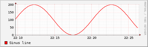
This is the one of most simple commands to use rrdtool to create a graph. This command will use defaults for all non-specified parameters.
$ rrdtool graph rrdtool1_graph1.png \
    --start now-1000s --end now \
    DEF:ds1a=dbfile1.rrd:ds1:AVERAGE \
    LINE1:ds1a#FF0000:"Sinus line"
This rrdtool command “graph” instructs rrdtool to create a graph followed by the file name of the image. The parameter “–start” and “–end” define the start and end time for the rrd graph in the same way as in the create command.
DEF:ds1a=dbfile1.rrd:ds1:AVERAGE
The relevant specification for the DEF line is “DEF:vname=rrdfile:ds-name:CF”.
- DEF – The line starting with “DEF” instructs rrdtool to fetch data from the rrd databse.
- ds1a – The vname is a virtual name for the retrieved data for later use.
- dbfile1.rrd – The filename of the rrd datase file to fetch the data from.
- ds1 – The ds-name for the dataset in the rrd database file as it was specified during creation of the rrd file.
- AVERAGE – The CF to be used if consolidation needs to be done while creating the graph.
With the data fetched from the rrd database file, rrdtool needs to be instructed what to do with this data points. There are different options to control how the data points are drawn. The example starts with a simple line.
LINE1:ds1a#FF0000:"Sinus line"
The relevant syntax for drawing a line is “LINE[width]:value[#color][:[legend]”
- LINE1 – Defines the way the data is drawn. In this example, as line with a line width of 1. The number can be increased to draw thicker lines.
- ds1a – The vname as defined in the DEF line above referencing the data from the file.
- #FF0000 – The color the line should be drawn at. The example define a red line.
- “Sinus line” – The name of the line shown in the legend of the graph.
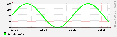
With a few small changes, the graph can be changed to look different. For example, increasing the number in “LINE1” to “LINE3” and changing the color code to “#00FF00” will draw a thicker line in green.
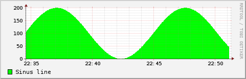
When the “LINE1” is replaced by “AREA”, the graph does not show a line, but shades the area that would have been under the line.
Read more of my posts on my blog at https://blog.tinned-software.net/.